
Countifs Not Working because your criteria range and sum range have different dimensions, which prevents the function from calculating correctly. Most of the time, this happens because the selected ranges don’t contain the same number of rows or columns. You can verify this quickly by selecting the ranges and checking the status bar in your spreadsheet software. If the counts don’t match, the software can’t align the cells, and it will return an error or an incorrect result. Always ensure your data sets are identical in size before you run the formula.
Why your Countifs isn’t working
| Cause | How common | How to confirm it | Fix it yourself? |
|---|---|---|---|
| Mismatched range sizes | Very common | Check row counts | Yes |
| Text wrapped in quotes | Common | Review formula syntax | Yes |
| Hidden trailing spaces | Common | Use TRIM function | Yes |
| Incorrect data types | Occasional | Check cell formatting | Yes |
| Calculation set manual | Rare | Check formula options | Yes |
| Corrupt cell references | Rare | Re-select data range | Yes |
| External sheet limits | Rare | Check workbook links | No |
Most users assume these errors stem from complex logic, but the vast majority of failures involve simple formatting mismatches. If your VLOOKUP returns #N/A despite a visual match, check the source cell for a leading space. A single hidden character renders the lookup value unique to the system.
If the formula returns a raw string instead of a result, ensure the cell isn’t formatted as “Text.” Excel will treat the formula as a literal sentence if the cell format is locked before you type the equals sign. To fix this, change the format to “General,” then re-enter the formula by pressing F2 followed by Enter.
When dealing with external links, verify if the source workbook is closed. If your calculation relies on a closed file, some complex array functions will fail to refresh. Always open the source file first to determine if the error is a broken path or a simple synchronization delay. If the error persists while the source file is open, the link path is likely corrupted.
Range size mismatch issues
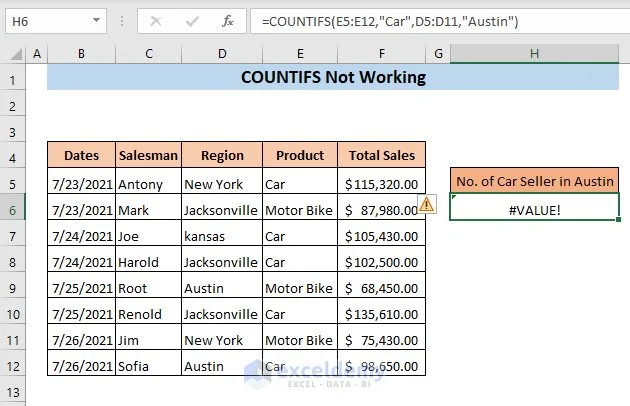
Mismatched range sizes occur when your criteria range and your sum range don’t align perfectly. The function requires every range provided to have the same number of rows and columns to map the data points accurately. If you define a criteria range as A1:A10 but your sum range as B1:B12, the system can’t process the extra two cells, leading to a calculation error.
To confirm this, highlight your first range and look at the bottom corner of your screen to see the count of selected rows. Repeat this for every range used in your formula. If the numbers differ, your ranges are incompatible. To fix this, adjust the cell references so that all ranges start and end on the same relative row numbers. For instance, if you use A1:A20, your second range must also be B1:B20.
This fix takes only a few seconds if you’re comfortable editing formulas in the bar. If you have many ranges, this can be tedious, but it’s necessary for the function to return a value. If you’re working with dynamic tables, consider using named ranges instead of static cell references. Named ranges automatically expand or contract with your data, which helps avoid this mismatch entirely. This varies by model — check the official Microsoft Excel support documentation for specific syntax rules regarding range alignment in your version of the software.
Syntax errors with criteria
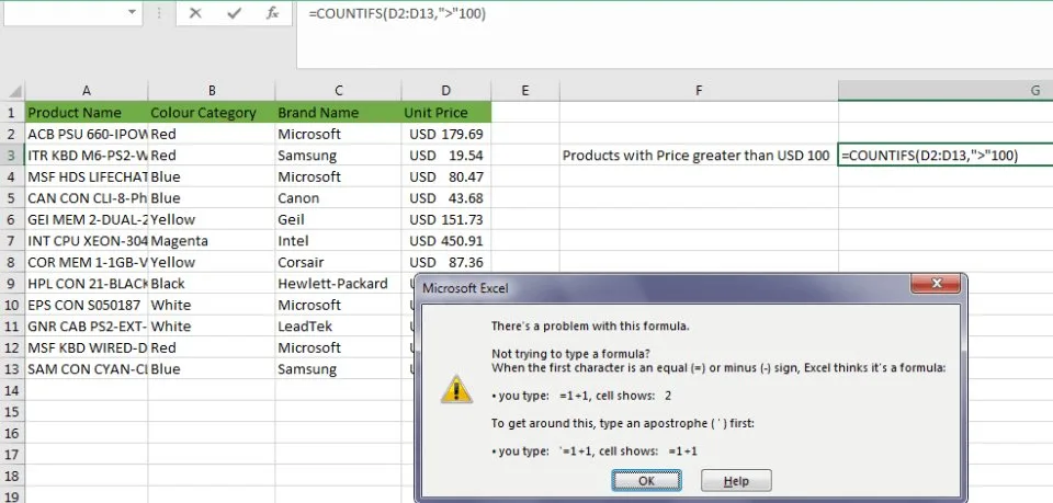
Syntax errors often stem from how you wrap criteria inside the function. When you use logical operators like greater than or less than, you must enclose the entire condition in double quotes. For example, typing “>50” tells the function to look for values higher than fifty. If you type >50 without the quotes, the software will return an error because it can’t interpret the symbol as a standalone value.
You can tell this is the cause if your formula displays a specific error message like #VALUE! or #N/A. To confirm, look closely at your formula bar. If you see a comparison operator sitting outside the quotes, that’s your mistake. To fix it, place the operator and the number inside the quotes, like this: “>50”. If you’re referencing a cell that contains the number, you must use an ampersand to join them, such as “>”&A1.
This is a common mistake that costs users time because it looks correct at a glance. If you don’t use the ampersand correctly when referencing a cell, the function will look for the literal text “>A1” instead of the value inside cell A1. This isn’t for users who prefer to avoid manual formula editing, as it requires careful attention to punctuation. If you find this difficult, use the “Insert Function” dialog box to build your criteria step by step, which prevents most quote-related errors.
Hidden formatting problems
Hidden spaces or mismatched data types often prevent the function from finding matches. A cell might look like it contains “Apple,” but it could actually hold “Apple ” with a trailing space. To the human eye, they look identical, but the software treats them as two different values. If you’re trying to count instances of “Apple,” the function will ignore the cell with the extra space.
To confirm this, select a cell you suspect is causing trouble and look at the formula bar. Click inside the bar and use your arrow keys to move to the end of the text. If the cursor stops one space to the right of the last letter, you have a trailing space. To fix this, use the TRIM function in a helper column to remove these extra spaces across your entire data set.
Another issue is when numbers are stored as text. This happens if you import data from a CSV file or a database. The function won’t count a number like 50 if the cell format is set to text. You can fix this by selecting the column, choosing the “Data” tab, and using “Text to Columns” to convert the data back to a number format. This is a simple task, but it requires you to know how your data was originally imported.
The less likely causes
Calculation settings in your software might be set to manual. If so, the sheet won’t update until you press the refresh key. Check the status bar at the bottom of your window; if it says “Calculate,” your sheet is paused.
The workbook might contain circular references. These stop the software from completing any calculations in the entire file. Look for a small error notification in the bottom-left corner of the status bar to identify the specific cell causing the loop.
You might have accidentally locked a cell reference with dollar signs. This prevents the formula from working correctly when you copy it down. If your results remain identical across rows, toggle the F4 key to remove the absolute references.
If your file is stored on a network drive, a lost connection stops the function from pulling data. If you see a file path starting with a backslash instead of a drive letter, your link is likely broken. Always map the drive locally to ensure stability.
If you need to access files on a protected server, you must contact your IT administrator. Without the correct database permissions, the software will return a generic error rather than a specific warning.
What a fix usually involves
Fixing a calculation error usually involves manual adjustments to your spreadsheet cells. If you have mismatched ranges, you’ll spend a small amount of time correcting the cell addresses in the formula bar. This costs nothing but your time. If you have hidden spaces, you’ll need to apply a formula to clean your data, which takes a few extra minutes but requires no new tools.
If your data is stored in a complex way, such as across multiple password-protected files, you may need to ask a colleague for the correct file path. Most fixes are simple, but if you’re dealing with a large database, you might need help from someone who understands data management. If you’re unsure about the state of your data, always save a backup copy of your file before you start changing formulas. You can check the current version of your software on the “About” screen to see if there are specific updates or patches that improve how functions behave.
Frequently asked questions
Can I use wildcards in my criteria?
Yes, you can use wildcards like the asterisk to represent any number of characters. For example, using “A*” will count all cells that start with the letter A. The asterisk acts as a placeholder for any text that follows. This is helpful when your data isn’t perfectly consistent but follows a specific pattern you can identify.
Why does my formula return zero?
Zero often means your criteria don’t match any cells in your range. Check your spelling, look for hidden spaces, and ensure your numbers aren’t formatted as text. If you’re certain the data is correct, try selecting a smaller range to see if the function works on a limited set of cells first.
Is it safe to use this function on large files?
Yes, it’s perfectly safe to use this function on large files, though it may slow down your machine if you have thousands of calculations running at once. If your computer freezes, try setting your calculation options to manual. This keeps the software from trying to update every single cell every time you make a small change.
What happens if I have multiple criteria?
The function will only count cells that meet every single condition you provide. If you have three criteria, a cell must satisfy all three to be included in the final count. If you need to count cells that meet any one of several conditions, you’ll need to use a different method.
Does it matter if I use uppercase or lowercase?
No, the function isn’t case-sensitive, so it will treat “apple” and “APPLE” as the same thing. You don’t need to worry about capitalization when you write your criteria. This makes it easier to work with data that might have been typed by different people in different styles.
How long does a fix take?
Most fixes take about five minutes once you identify the problem. If you have a large data set that requires cleaning, it might take a bit longer, but the process remains the same. You’re simply removing spaces or correcting ranges, which are straightforward tasks that don’t require advanced technical skills.
Final Thoughts
Checking your data alignment is a simple habit that saves a lot of frustration later on. Once you’ve fixed these range sizes, try applying the same logic to your other complex formulas. You’ll find that your spreadsheets run much smoother when you’re confident that every cell matches up perfectly.